One of the most important properties in Neural Networks is to improve performance by learning from past experiences. Learning is a process where a network learns through an interactive process of applied parameters. The network becomes more knowledgeable in every iteration of the learning process. Before we go ahead and see how the learning actually happens in detail, lets take a look at two important parameters that will play a major role in learning.
Weights and Biases
Weight and bias are learning parameters that transform input data within the networks hidden layers. Both of these parameters are adjusted during training. Weight affects the amount of influence a change in the input will have upon the output while Bias mainly represents how far off the predictions are from the actual values.
 source DeepAi
Learning Process
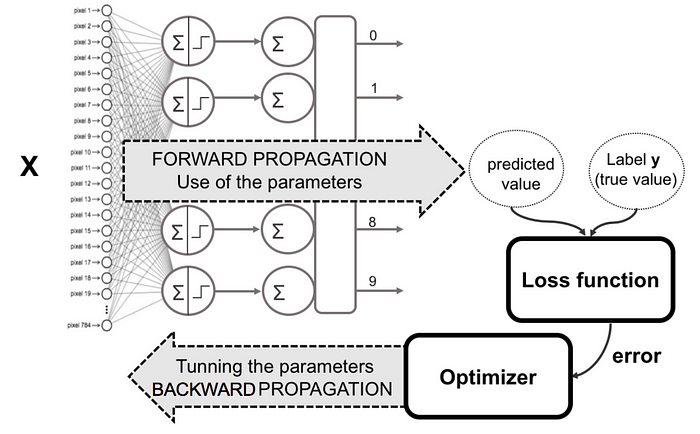
Neural networks are composed of layers of neurons (computational units) connected to each other. Each neuron transforms input data by multiplying the initial values by weights. The neurons have an activation function that defines the neurons output. The activation function is used to introduce non-linearity in the model and ensures that values passed in the network lie within the expected range. This process is repeated until the final output layer can provide predictions related to the task. Neural networks build knowledge from datasets where the right answer is provided in advance, then learn by tuning themselves to find the answers on their own in an iterating process of going 'back and forth' increasing the accuracy of predictions. The process of going 'forth' is called forward propagation, while the going 'back' is called back propagation.
Activation Function
Activation function is an algorithm used in neural networks which defines how the weighted sum of the input values is transformed into outputs. Activation functions are useful as they add non-linearity to the network. Non-linearity means that the output cannot be reproduced from a linear combination of inputs. Non-Linear functions are useful as they help networks learn complex information in order to provide accurate predictions/outputs. The reason we use non linear activation functions is because if we were to use a linear activation function then the neural network will just produce a linear function of inputs and no matter how many layers our neural network has, it will behave just like a single layer.
Let's look at some of the commonly used non-linear activation functions.
Sigmoid
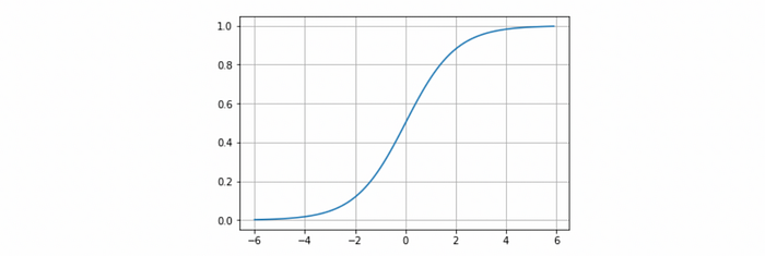
sigmoid function also know as 'logistic function' takes any real value as input and outputs values between 0 and 1.The greater the input, the closer the output will be to 1 and the smaller the input, the closer the output will be to 0.Sigmoid gives an 'S' shape. see example below

SoftMax
SoftMax functions is usually used for the output layer in neural networks that need to classify inputs to multiple categories. It returns the probability distributions of output classes by normalizing each class output to values between 0 and 1 and divides by their sum giving the probability of the input value being in a specific class.
Forward Propagation
Forward propagation is the process where the input data is passed into the network where by all neurons apply their transformation(activation function) to the data they received from the previous layer of neurons and pass it to the next layer. The data flows in a forward direction till the final layer is reached and produces the output data(predictions). The input data is fed only in a forward direction and the data does not flow in reverse direction during the generation of the output data. These configurations are known as feed-forward networks which help in forward propagation. The reason why the data needs to only flow forward is because the reverse direction will cause a formation of a cycle thereby prohibiting the generating of output data(that's why they are called feed forward networks).
Loss Functions
The next phase is to use the loss function to estimate the errors and measure the models predictions against the actual values. A loss function is a method used to optimize models with the intent of reducing the loss between predicted values and actual values. Ideally we want as less loss as possible, that is why it is important to adjust the parameters gradually till we achieve the desired results.
Back Propagation
Once the loss has been calculated the information is then propagated backward hence getting the name back propagation. It involves the calculation of the gradient going back ward through the feed forward network from the last layer to the first. This allows us to calculate the gradient of the loss function with respect to the weights of the model. Weights are updated individually to gradually reduce the loss function over training iterations. see image below
 source toress.ai
What this process above represents is that we are making the loss as low as possible when we go back to iterating to the network. This technique is called gradient descent.
Gradient Descent
Gradient descent is an optimization algorithm used to train models by minimizing the loss function whenever the parameters are being updated. Until the loss function is close to zero or equal to, the model continues to adjust in order for the parameters to obtain as minimum as possible. In order for the gradient to reach a minimum, the learning rate should be set at an appropriate value. If the learning rate is too high, the minimum point will not be reached but if we set the learning rate too low the gradient will take time to reach the minimum point, that is why the learning rate shouldn't be too high or too low.
Let's look at the type of gradient descents
Batch Gradient Descent
Batch gradient descent calculates the error of each example within the training dataset but only updates the parameters after all the training examples have been evaluated. The advantage of batch gradient descent is that it is computationally efficient, produces stable error gradient and a stable convergence, but sometimes that convergence point isn’t the best the model can achieve.
Stochastic Gradient Descent
Stochastic gradient descent (SGD) runs a training epoch for each example within the dataset and it updates each training example's parameters one at a time. The advantage of SDG is that it's frequent updates allows us to have a pretty detailed rate of improvement but because of the frequent updates it becomes more computationally expensive than batch gradient descent.
Mini-batch Gradient Descent
Mini-batch gradient descent combines both batch gradient descent and stochastic gradient descent concepts. It splits the training dataset into small batch sizes and performs updates on each of those batches. This approach strikes a balance between the computational efficiency of batch gradient descent and the speed of stochastic gradient descent. This is the go-to algorithm when training a neural network and it is the most common type of gradient descent within deep learning.
Overfitting
Overfitting is a concept in machine learning where the model fits exactly against the training data and doesn't perform well when it comes to unseen data. Generally we want models to perform well for both training and testing data(unseen data). Overfitting happens when the model trains for too long and starts to memorize the data. Low error rate and high accuracy in a model are good indicators of model over fitting. see example below
 example of an overfitting model source Wikipedia
There are a few methods one can try to avoid overfitting :
- Less training - reducing the training epochs or training time helps with overfitting by reducing the model noise and preventing the model in memorizing the data.
- Reducing Neural Layers - A complex model is likely to overfitting therefore by reducing the neural network layers, the model becomes less complex and eventually reducing overfitting.
- Dropout - Dropout is a form of regularization, a technique used to constrain models from learning complex data. Applying dropout helps by reducing or randomly ignoring neurons in a given layer during training hence reducing overfitting.
Conclusion
Finally deep learning plays a crucial role in our modern civilization. From demographic statistics to healthcare, deep learning has been a tool that enabled devising of viable solutions to address real life problems. It is very important for those that want to delve into this pool of unlimited knowledge to have a full comprehension of it, starting from the basics provided. With these few basic insights, l believe one is able to navigate a way to advance and create a brighter future that we all hope for with a magic touch of AI.
If you missed the previous sections of this article you can find

